Quickstart
Defining the orbit: Orbit objects
The core of poliastro are the Orbit objects
inside the poliastro.twobody module. They store all the required
information to define an orbit:
The body acting as the central body of the orbit, for example the Earth.
The position and velocity vectors or the orbital elements.
The time at which the orbit is defined.
First of all, we have to import the relevant modules and classes:
from astropy import units as u

from poliastro.bodies import Earth, Mars, Sun
from poliastro.twobody import Orbit
From position and velocity
There are several methods available to create
Orbit objects. For example, if we have the
position and velocity vectors we can use
from_vectors():
# Data from Curtis, example 4.3
r = [-6045, -3490, 2500] * u.km
v = [-3.457, 6.618, 2.533] * u.km / u.s

orb = Orbit.from_vectors(Earth, r, v)
And that’s it! Notice a couple of things:
Defining vectorial physical quantities using Astropy units is very easy. The list is automatically converted to a
astropy.units.Quantity, which is actually a subclass of NumPy arrays.
If we display the orbit we just created, we get a string with the radius of pericenter, radius of apocenter, inclination, reference frame and attractor:
>>> orb
7283 x 10293 km x 153.2 deg (GCRS) orbit around Earth (♁) at epoch J2000.000 (TT)
If no time is specified, then a default value is assigned:
>>> orb.epoch
<Time object: scale='tt' format='jyear_str' value=J2000.000>
>>> orb.epoch.iso
'2000-01-01 12:00:00.000'
The reference frame of the orbit will be one pseudo-inertial frame around the attractor. You can retrieve it using the
frameproperty:orb.get_frame() <GCRS Frame (obstime=J2000.000, obsgeoloc=(0., 0., 0.) m, obsgeovel=(0., 0., 0.) m / s)>
Intermezzo: quick visualization of the orbit
If we’re working on interactive mode (for example, using the wonderful Jupyter notebook) we can immediately plot the current orbit:
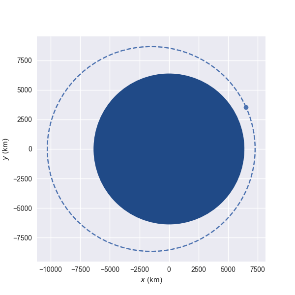
orb.plot()
This plot is made in the so called perifocal frame, which means:
we’re visualizing the plane of the orbit itself,
the $(x)$ axis points to the pericenter, and
the $(y)$ axis is turned $90 \mathrm{^\circ}$ in the direction of the orbit.
The dotted line represents the osculating orbit: the instantaneous Keplerian orbit at that point. This is relevant in the context of perturbations, when the object shall deviate from its Keplerian orbit.
Note
This visualization uses Plotly under the hood and works best in a Jupyter notebook.
To use the static interface based on matplotlib, which might be more useful for batch jobs and ublication-quality plots, check out the poliastro.plotting.static.StaticOrbitPlotter.
From classical orbital elements
We can also define an Orbit using a set of
six parameters called orbital elements. Although there are several of these element sets, each one with its advantages and drawbacks, right now poliastro supports the classical orbital elements:
Semimajor axis $(a)$.
Eccentricity $(e)$.
Inclination $(i)$.
Right ascension of the ascending node $(\Omega)$.
Argument of pericenter $(\omega)$.
True anomaly $(\nu)$.
In this case, we’d use the method
from_classical():
# Data for Mars at J2000 from JPL HORIZONS
a = 1.523679 * u.AU
ecc = 0.093315 * u.one
inc = 1.85 * u.deg
raan = 49.562 * u.deg
argp = 286.537 * u.deg
nu = 23.33 * u.deg

orb = Orbit.from_classical(Sun, a, ecc, inc, raan, argp, nu)
Notice that whether we create an Orbit from $(r)$ and $(v)$ or from
elements we can access many mathematical properties of the orbit:
>>> orb.period.to(u.day)
<Quantity 686.9713888628166 d>
>>> orb.v
<Quantity [  1.16420211, 26.29603612,  0.52229379] km / s>
To see a complete list of properties, check out the
poliastro.twobody.orbit.Orbit class on the API reference.
Moving forward in time: propagation
Now that we have defined an orbit, we might be interested in computing how is it going to evolve in the future. In the context of orbital mechanics, this process is known as propagation, and can be performed with the propagate method of Orbit objects:
>>> from poliastro.examples import iss
>>> iss
6772 x 6790 km x 51.6 deg (GCRS) orbit around Earth (♁)
>>> iss.epoch
<Time object: scale='utc' format='iso' value=2013-03-18 12:00:00.000>
>>> iss.nu.to(u.deg)
<Quantity 46.595804677061956 deg>
>>> iss.n.to(u.deg / u.min)
<Quantity 3.887010576192155 deg / min>
Using the propagate() method we can now retrieve the position of the ISS after some time:
>>> iss_30m = iss.propagate(30 * u.min)
>>> iss_30m.epoch  # Notice we advanced the epoch!
<Time object: scale='utc' format='iso' value=2013-03-18 12:30:00.000>
>>> iss_30m.nu.to(u.deg)
<Quantity 163.1409357544868 deg>
For more advanced propagation options, check out the
poliastro.twobody.propagation module.
Studying non-keplerian orbits: perturbations
Apart from the Keplerian propagators, poliastro also allows the user to define custom perturbation accelerations to study non Keplerian orbits, thanks to Cowell’s method:
>>> from numba import njit
>>> import numpy as np
>>> from poliastro.core.propagation import func_twobody
>>> from poliastro.twobody.propagation import cowell
>>> r0 = [-2384.46, 5729.01, 3050.46] * u.km
>>> v0 = [-7.36138, -2.98997, 1.64354] * u.km / u.s
>>> initial = Orbit.from_vectors(Earth, r0, v0)
>>> @njit
... def accel(t0, state, k):
...     """Constant acceleration aligned with the velocity. """
...     v_vec = state[3:]
...     norm_v = (v_vec * v_vec).sum() ** 0.5
...     return 1e-5 * v_vec / norm_v
...
... def f(t0, u_, k):
...     du_kep = func_twobody(t0, u_, k)
...     ax, ay, az = accel(t0, u_, k)
...     du_ad = np.array([0, 0, 0, ax, ay, az])
...     return du_kep + du_ad

>>> initial.propagate(3 * u.day, method=cowell, f=f)
18255 x 21848 km x 28.0 deg (GCRS) orbit around Earth (♁) at epoch J2000.008 (TT)
Some natural perturbations are available in poliastro to be used directly in this way. For instance, let us examine the effect of J2 perturbation:
>>> from poliastro.core.perturbations import J2_perturbation
>>> tofs = [48.0] * u.h
>>> def f(t0, u_, k):
...     du_kep = func_twobody(t0, u_, k)
...     ax, ay, az = J2_perturbation(
...         t0, u_, k, J2=Earth.J2.value, R=Earth.R.to(u.km).value
...     )
...     du_ad = np.array([0, 0, 0, ax, ay, az])
...     return du_kep + du_ad

>>> final = initial.propagate(tofs, method=cowell, f=f)
The J2 perturbation changes the orbit parameters (from Curtis example 12.2):
>>> ((final.raan - initial.raan) / tofs).to(u.deg / u.h)
<Quantity -0.17232668 deg / h>
>>> ((final.argp - initial.argp) / tofs).to(u.deg / u.h)
<Quantity 0.28220397 deg / h>
For more available perturbation options, see the poliastro.twobody.perturbations module.
Studying artificial perturbations: thrust
In addition to natural perturbations, poliastro also has built-in artificial perturbations (thrusts) aimed at intentional change of some orbital elements. Let us simultaneously change eccentricity and inclination:
>>> ecc_0, ecc_f = 0.4, 0.0
>>> a = 42164  # km
>>> inc_0 = 0.0  # rad, baseline
>>> inc_f = 20.0 * u.deg
>>> argp = 0.0  # rad, the method is efficient for 0 and 180
>>> f = 2.4e-7 * (u.km / u.s ** 2)

# Retrieve r and v from initial orbit
>>> s0 = Orbit.from_classical(
...     Earth,
...     a * u.km,
...     ecc_0 * u.one,
...     inc_0 * u.deg,
...     0 * u.deg,
...     argp * u.deg,
...     0 * u.deg,
... )
>>> a_d, _, t_f = change_ecc_inc(s0, ecc_f, inc_f, f)

# Propagate orbit
>>> def f_geo(t0, u_, k):
...     du_kep = func_twobody(t0, u_, k)
...     ax, ay, az = a_d(t0, u_, k)
...     du_ad = np.array([0, 0, 0, ax, ay, az])
...     return du_kep + du_ad

>>> sf = s0.propagate(t_f * u.s, method=cowell, f=f_geo, rtol=1e-8)
The thrust changes orbit parameters as desired (within errors):
>>> sf.inc, sf.ecc
(<Quantity 0.34719734 rad>, <Quantity 0.00894513>)
For more available perturbation options, see the
poliastro.twobody.thrust module.
Changing the orbit: Maneuver objects
poliastro helps us define several in-plane and general out-of-plane
maneuvers with the Maneuver class inside the
poliastro.maneuver module.
Each Maneuver consists on a list of impulses $\Delta v_i$ (changes in velocity) each one applied at a certain instant $t_i$. The simplest maneuver is a single change of velocity without delay: you can
recreate it either using the impulse() method or instantiating it directly.
from poliastro.maneuver import Maneuver

dv = [5, 0, 0] * u.m / u.s

man = Maneuver.impulse(dv)
man = Maneuver((0 * u.s, dv))  # Equivalent
There are other useful methods you can use to compute common in-plane maneuvers, notably {py:meth} ~poliastro.maneuver.Maneuver.hohmann and bielliptic() for Hohmann and bielliptic transfers respectively. Both return the corresponding Maneuver object, which in turn you can use to calculate the total cost
in terms of velocity change $\sum |\Delta v_i|$ and the transfer time:
>>> ss_i = Orbit.circular(Earth, alt=700 * u.km)
>>> ss_i
7078 x 7078 km x 0.0 deg (GCRS) orbit around Earth (♁)
>>> hoh = Maneuver.hohmann(ss_i, 36000 * u.km)
>>> hoh.get_total_cost()
<Quantity 3.6173981270031357 km / s>
>>> hoh.get_total_time()
<Quantity 15729.741535747102 s>
You can also retrieve the individual vectorial impulses:
>>> hoh.impulses[0]
(<Quantity 0 s>, <Quantity [ 0.        , 2.19739818, 0.        ] km / s>)
>>> hoh[0]  # Equivalent
(<Quantity 0 s>, <Quantity [ 0.        , 2.19739818, 0.        ] km / s>)
>>> tuple(val.decompose([u.km, u.s]) for val in hoh[1])
(<Quantity 15729.741535747102 s>, <Quantity [ 0.        , 1.41999995, 0.        ] km / s>)
To actually retrieve the resulting Orbit after performing a maneuver, use
the method apply_maneuver():
>>> ss_f = ss_i.apply_maneuver(hoh)
>>> ss_f
36000 x 36000 km x 0.0 deg (GCRS) orbit around Earth (♁)
More advanced plotting: OrbitPlotter* objects
We previously saw the plot() method to easily plot orbits. Now we’d like to plot several orbits in one graph (for example, the maneuver we computed in the previous section). For this purpose, we have OrbitPlotter* objects in the plotting module.
These objects hold the perifocal plane of the first Orbit we plot in them, projecting any further trajectories on this plane. This allows to easily visualize in two dimensions:
from poliastro.plotting import OrbitPlotter2D

op = OrbitPlotter2D()
ss_a, ss_f = ss_i.apply_maneuver(hoh, intermediate=True)
op.plot(ss_i, label="Initial orbit")
op.plot(ss_a, label="Transfer orbit")
op.plot(ss_f, label="Final orbit")
Which produces this beautiful plot:
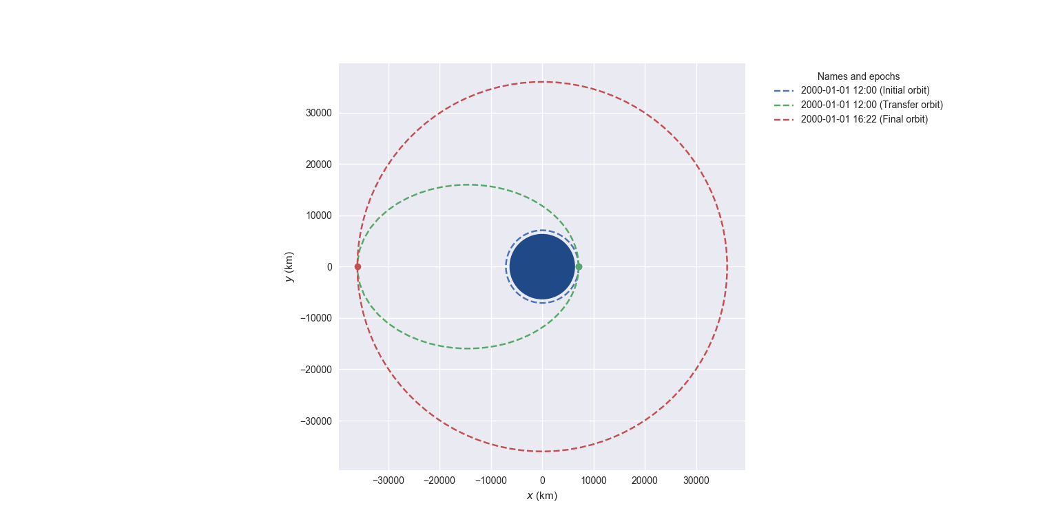
Plot of a Hohmann transfer.
Where are the planets? Computing ephemerides
New in version 0.14.0.
Thanks to Astropy and jplephem, poliastro can read Satellite Planet Kernel (SPK) files, part of NASA’s SPICE toolkit. This means that we can query the position and velocity of the planets of the Solar system.
The poliastro.ephem.Ephem class allows us to retrieve
a planetary orbit using low precision ephemerides available in Astropy and an astropy.time.Time:
from astropy import time
epoch = time.Time("2020-04-29 10:43")  # UTC by default
And finally, retrieve the planet ephemerides:
>>> from poliastro.ephem import Ephem
>>> earth = Ephem.from_body(Earth, epoch.tdb)
>>> earth
Ephemerides at 1 epochs from 2020-04-29 10:44:09.186 (TDB) to 2020-04-29 10:44:09.186 (TDB)
This does not require any external download. If on the other hand we want to use higher precision ephemerides, we can tell Astropy to do so:
>>> from astropy.coordinates import solar_system_ephemeris
>>> solar_system_ephemeris.set("jpl")
Downloading http://naif.jpl.nasa.gov/pub/naif/generic_kernels/spk/planets/de430.bsp
|==========>-------------------------------|  23M/119M (19.54%) ETA    59s22ss23
This in turn will download the ephemerides files from NASA and use them for future computations. For more information, check out Astropy documentation on ephemerides.
Warning
This is the preferred method over poliastro.twobody.orbit.Orbit.from_body_ephem(), which is now deprecated and will be removed in the next release.
If we want to retrieve the osculating orbit at a given epoch,
we can do so using from_ephem():
>>> Orbit.from_ephem(Sun, earth, epoch)
1 x 1 AU x 23.4 deg (HCRS) orbit around Sun (☉) at epoch 2020-04-29 10:43:00.000 (UTC)
Note
Notice that the position and velocity vectors are given with respect to the Heliocentric Celestial Reference System (HCRS) which means equatorial coordinates centered on the Sun.
Traveling through space: solving the Lambert problem
The determination of an orbit given two position vectors and the time of flight is known in celestial mechanics as Lambert’s problem, also known as two point boundary value problem. This contrasts with Kepler’s problem or propagation, which is rather an initial value problem.
The package poliastro.iod holds the different raw algorithms to solve Lambert’s problem, provided the main attractor’s gravitational constant, the two position vectors and the time of flight. As you can imagine, being able to compute the positions of the planets as we saw in the previous section is the
perfect complement to this feature!
Since poliastro version 0.13 it is possible to solve Lambert’s problem by making use of the poliastro.maneuver module. We just need to pass as arguments the initial and final orbits and the output will be a poliastro.maneuver.Maneuver instance. Time of flight is computed internally since orbits epochs are known.
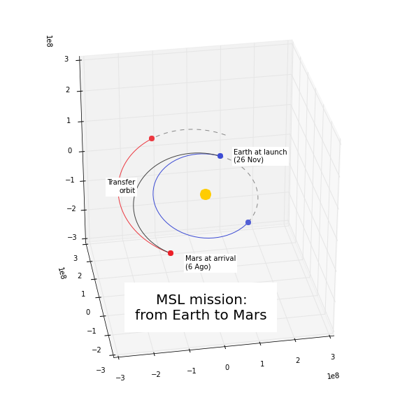
For instance, this is a simplified version of the example “Going to Mars with Python using poliastro”, where the orbit of the Mars Science Laboratory mission (rover Curiosity) is determined:
date_launch = time.Time('2011-11-26 15:02', scale='tdb')
date_arrival = time.Time('2012-08-06 05:17', scale='tdb')

ss0 = Orbit.from_ephem(Sun, Ephem.from_body(Earth, date_launch), date_launch)
ssf = Orbit.from_ephem(Sun, Ephem.from_body(Mars, date_arrival), date_arrival)

man_lambert = Maneuver.lambert(ss0, ssf)
dv_a, dv_b = man_lambert.impulses
And these are the results:
>>> dv_a
(<Quantity 0. s>, <Quantity [-2.06420561,  2.58796837,  0.23911543] km / s>)
>>> dv_b
(<Quantity 21910501.00019529 s>, <Quantity [287832.91384349,  58935.96079319, -94156.93383463] km / s>)
Fetching Orbits from external sources
As of now, poliastro supports fetching orbits from 2 online databases from Jet Propulsion Laboratory: SBDB and Horizons.
JPL Horizons can be used to generate ephemerides for solar-system bodies, while JPL SBDB (Small-Body Database Browser) provides model orbits for all known asteroids and many comets.
The data is fetched using the wrappers to these services provided by astroquery:
epoch = time.Time("2020-04-29 10:43")
Ephem.from_horizons("Ceres", epoch)
Orbit.from_sbdb("Apophis")
Creating a CZML document
We can create CZML documents which can then be visualized with the help of Cesium.
First we load the orbital data and the CZML Extractor:
from poliastro.examples import molniya, iss
from poliastro.czml.extract_czml import CZMLExtractor
Then we specify the starting and ending epoch, as well as the number of sample points (the higher the number, the more accurate the trajectory):
start_epoch = iss.epoch
end_epoch = iss.epoch + molniya.period
sample_points = 10

extractor = CZMLExtractor(start_epoch, end_epoch, sample_points)

extractor.add_orbit(molniya, label_text="Molniya")
extractor.add_orbit(iss, label_text="ISS")
We can find the generated CZML file by calling extractor.packets.
There is more information in this sample Cesium
application.
Per Python ad astra ;)