Studying Hohmann transfers

from astropy import units as u

from matplotlib import pyplot as plt
import numpy as np

from poliastro.bodies import Earth
from poliastro.maneuver import Maneuver
from poliastro.twobody import Orbit
from poliastro.util import norm

Earth.k

$3.9860044 \times 10^{14} \; \mathrm{\frac{m^{3}}{s^{2}}}$

ss_i = Orbit.circular(Earth, alt=800 * u.km)
ss_i

7178 x 7178 km x 0.0 deg (GCRS) orbit around Earth (♁) at epoch J2000.000 (TT)

r_i = ss_i.a.to(u.km)
r_i

$7178.1366 \; \mathrm{km}$

v_i_vec = ss_i.v.to(u.km / u.s)
v_i = norm(v_i_vec)
v_i

$7.4518315 \; \mathrm{\frac{km}{s}}$

N = 1000
dv_a_vector = np.zeros(N) * u.km / u.s
dv_b_vector = dv_a_vector.copy()
r_f_vector = r_i * np.linspace(1, 100, num=N)
for ii, r_f in enumerate(r_f_vector):
    man = Maneuver.hohmann(ss_i, r_f)
    (_, dv_a), (_, dv_b) = man.impulses
    dv_a_vector[ii] = norm(dv_a)
    dv_b_vector[ii] = norm(dv_b)

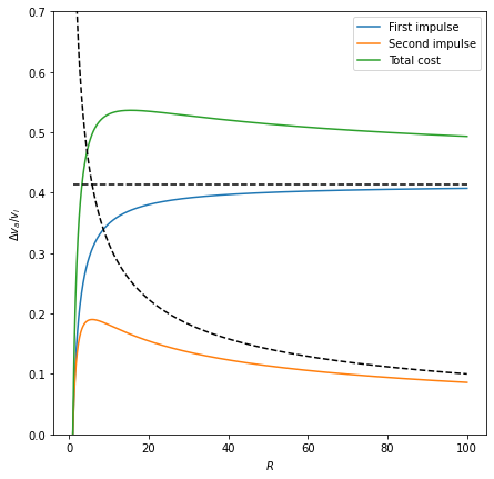
fig, ax = plt.subplots(figsize=(7, 7))

ax.plot((r_f_vector / r_i).value, (dv_a_vector / v_i).value, label="First impulse")
ax.plot((r_f_vector / r_i).value, (dv_b_vector / v_i).value, label="Second impulse")
ax.plot((r_f_vector / r_i).value, ((dv_a_vector + dv_b_vector) / v_i).value, label="Total cost")

ax.plot((r_f_vector / r_i).value, np.full(N, np.sqrt(2) - 1), 'k--')
ax.plot((r_f_vector / r_i).value, (1 / np.sqrt(r_f_vector / r_i)).value, 'k--')

ax.set_ylim(0, 0.7)
ax.set_xlabel("$R$")
ax.set_ylabel("$\Delta v_a / v_i$")

plt.legend()
fig.savefig("hohmann.png")